Summary: Simple plots in Rubyplot.

Table of Contents

• Introduction
• Scatter plot
• Area plot
• Bar plot
• Bubble plot
• Candle-stick plot
• Histogram
• Line plot
• Error-bar plot
• Box plot

Introduction

This blog lists down the simple plots in Rubyplot with ImageMagick as backend and highlights the work done in Week 3 and 4 for GSoC 2019.
P.S. - The version of Rubyplot used in this blog is dated 28th June.

Scatter plot

An example of Scatter plot with code is:

@x1 = [1, 2, 3, 4, 5]
@y1 = [11, 2, 33, 4, 65]
@figure = Rubyplot::Figure.new
axes = @figure.add_subplot! 0,0
axes.scatter! do |p|
  p.data @x1, @y1
  p.label = "data1"
  p.marker_size = 3
  p.marker_fill_color = :blue
  p.marker_type = :diagonal_cross
end
axes.title = "Scatter plot"
axes.x_title = "X data"
axes.y_title = "Y data"
@figure.write('scatterplot.png')

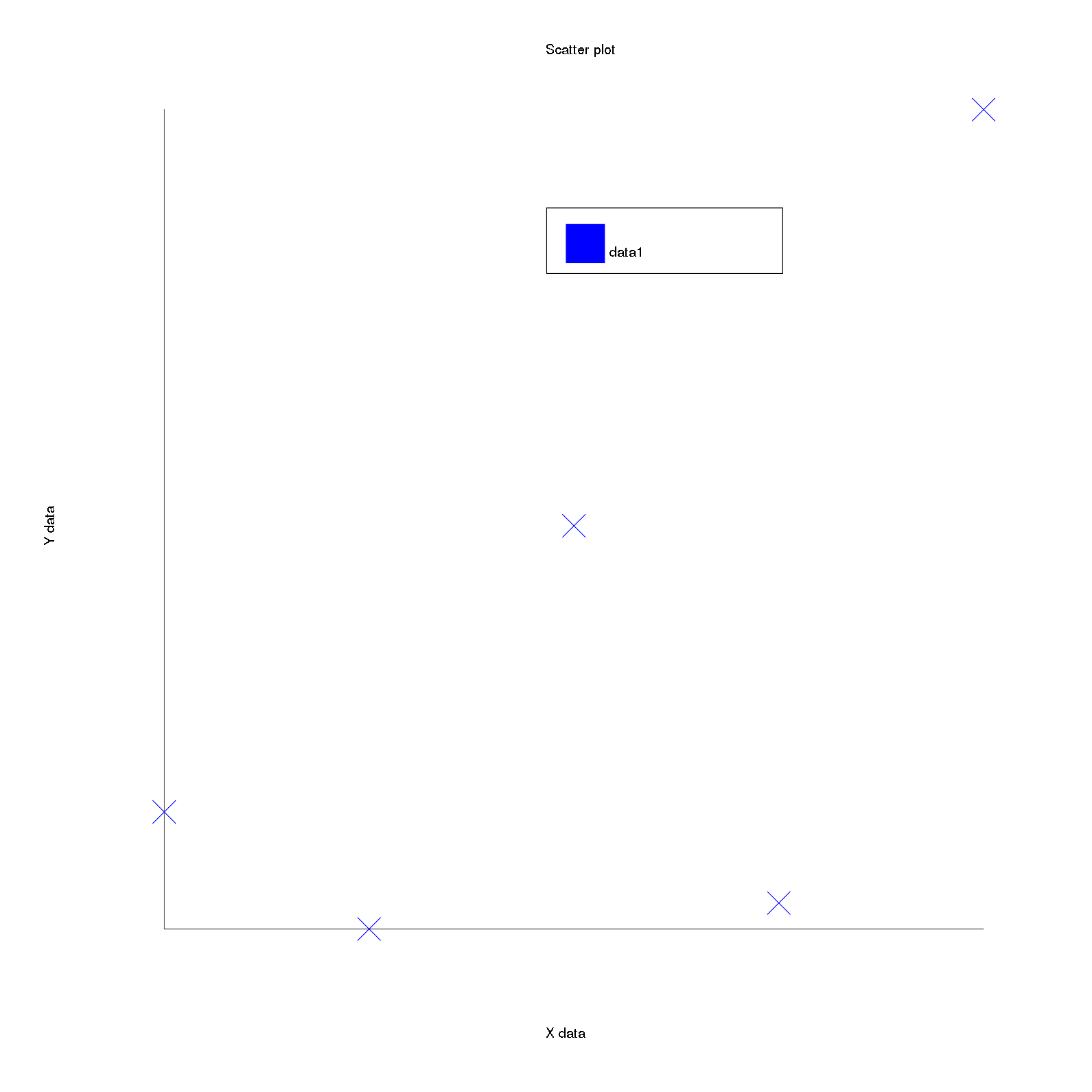
The scatter plot draws markers at the position specified by the user, the inputs taken are the X and Y coordinates for the markers (data), the label(label) for this plot, size of the marker (marker_size), type of the marker (marker_type), colour of the border of the marker (marker_border_color) and colour to be filled inside the marker (marker_fill_color).
If the marker does not have a fill colour (example - plus, diagonal cross, dot) then the fill colour is set as the colour of the colour of the marker.

draw function for scatter plot is:

def draw
  @marker_fill_color = :default if @marker_fill_color.nil?
  Rubyplot.backend.draw_markers(
    x: @data[:x_values],
    y: @data[:y_values],
    type: @marker_type,
    fill_color: @marker_fill_color,
    border_color: @marker_border_color,
    size: [@marker_size] * @data[:x_values].size
  )
end

Here, first the marker fill colour is set to default colour if it is nil the the draw_markers function is called:

def draw_markers(x:, y:, type: :default, fill_color: :default, border_color: :default, size: nil)
  y.each_with_index do |iy, idx_y|
    ix = transform_x(x: x[idx_y],abs: false)
    iy = transform_y(y: iy, abs: false)
    # in GR backend size is multiplied by
    # nominal size generated on the graphics device
    # so set the nominal_factor to 15
    within_window do
      size[idx_y] *= NOMINAL_FACTOR_MARKERS
      MARKER_TYPES[type].call(@draw, ix, iy, fill_color, border_color, size[idx_y])
    end
  end
end

The coordinates are first transformed, then the size of the marker is multiplied by a nominal factor (hardcoded to 15) to match the marker sizes in GR backend as GR backend multiplies its marker sizes by a nominal factor which is not mentioned.
To draw the markers, a hash is used which has lambdas for drawing different types of markers, an example of the hash is:

MARKER_TYPES = {
  # Default type is circle
  # Stroke width is set to 1
  default: ->(draw, x, y, fill_color, border_color, size) {
    draw.stroke Rubyplot::Color::COLOR_INDEX[border_color]
    draw.fill Rubyplot::Color::COLOR_INDEX[fill_color]
    draw.circle(x,y, x + size,y)
  },
  circle: ->(draw, x, y, fill_color, border_color, size) {
    draw.stroke Rubyplot::Color::COLOR_INDEX[border_color]
    draw.fill Rubyplot::Color::COLOR_INDEX[fill_color]
    draw.circle(x,y, x + size,y)
  },
  plus: ->(draw, x, y, fill_color, border_color, size) {
    # size is length of one line
    draw.stroke Rubyplot::Color::COLOR_INDEX[fill_color]
    draw.line(x - size/2, y, x + size/2, y)
    draw.line(x, y - size/2, x, y + size/2)
  }
  # Rest of the code omitted due to space constraint
}

Each of these lambdas take the properties of the marker and draw it depending on the type of marker, for example the circle type draws a circle with size as its radius, the plus type draws two perpendicular lines in the shape of a plus sign (+) with the size as length of the lines.
A hash of lambdas is used instead of making a module or a class to avoid inconsistencies in backends as GR does not require functions for creating marker types and only requires the type of the marker, i.e. its internal functions take care of drawing the marker types. Also, generally Hashes are much faster than functions and hence hashes are preferred over a module or a class.

Marker types implemented till now for ImageMagick bacckend are: circle, plus, dot, diagonal_cross, solid_circle, traingle_down, solid_traingle_down, traingle_up, solid_traingle_up, square, solid_square, bowtie, solid_bowtie, hglass, solid_hglass, diamond, solid_diamond, solid_tri_right, solid_tri_left, hollow_plus, solid_plus, vline, hline, omark.

Marker types not yet implemented for ImageMagick backend are: star, solid_star, asterisk, tri_up_down, pentagon, hexagon, heptagon, octagon, star_4, star_5, star_6, star_7, star_8.

Area plot

An example of Area plot with code is:

@figure = Rubyplot::Figure.new
axes = @figure.add_subplot! 0,0
axes.area! do |p|
  p.data [30, 36, 86, 39, 27, 31, 79, 88]
  p.label = "Jimmy"
end
axes.title = "Area plot"
@figure.write('areaplot.png')

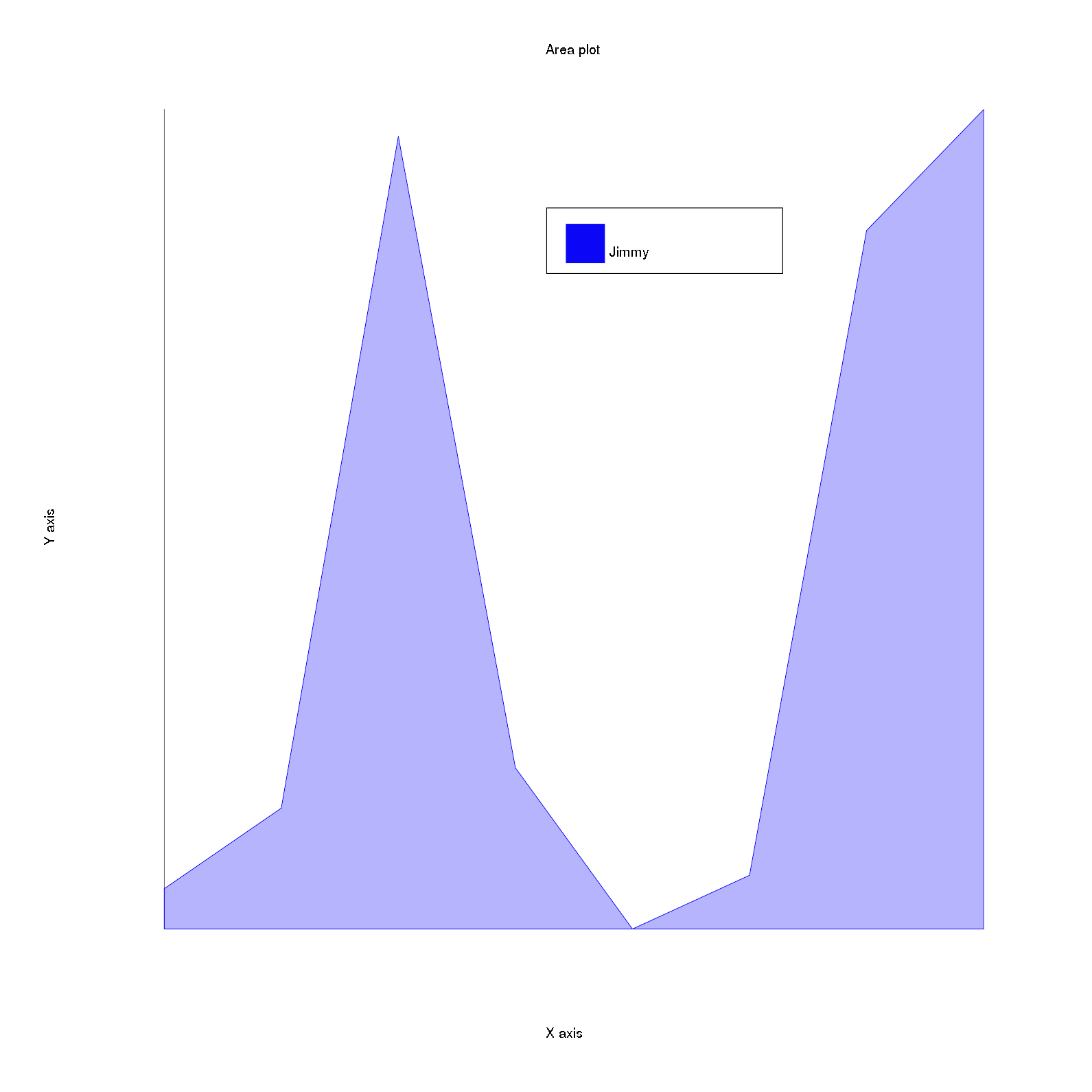
The area plot draws a line passing through the points given as the input and colours the area covered under this line.
The inputs taken are the data as a compulsory array containing Y coordinate values of the points and an optional array containing X coordinate values of the points(data), the label of the plot(label) and the color of the plot(color).

If only one set of values is given to the area plot as the data, for example only [30, 36, 86, 39, 27, 31, 79, 88] is given then this set is considered as a set of Y coordinates of the points and X coordinates are set as 0, 1, 2 … (size of y values - 1) i.e. the coordinates are (0, 30), (1, 36), (2, 86), (3, 39), (4, 27), (5, 31), (6, 79), (7, 88).

Now, this is the list of coordinates through which the line has to pass and the area under the curve is to be filled, but to draw this a polygon is needed in which the colour will be filled. TO create this polygon, we just need to append the starting point and end point of the X axis so that the polygon is completed. So, here in the example taken above the starting point of X axis is (minimum x value, minimum y value) i.e. (0, 27) and the end point of X axis is (maximum x value, minimum y value) i.e. (7, 27).
So, finally the coordinates for the polygon are (0, 30), (1, 36), (2, 86), (3, 39), (4, 27), (5, 31), (6, 79), (7, 88), (0, 27), (7, 27).
The code for appending these points is:

x_poly_points = @data[:x_values].concat([@axes.x_axis.max_val, @axes.x_axis.min_val])
y_poly_points = @data[:y_values].concat([@axes.y_axis.min_val, @axes.y_axis.min_val])

The opacity of the polygon i.e. the area under the curve is set to 0.3 to make the areas behind an area visible.
After this, a Rubyplot::Artist::Polygon object is created whhich uses the draw_polygon backend function to draw the polygon, the draw_polygon function is:

def draw_polygon(x:, y:, border_width:, border_type:, border_color:, fill_color:,
  fill_opacity:)
  within_window do
    x = x.map! { |ix| transform_x(x: ix, abs: false) }
    y = y.map! { |iy| transform_y(y: iy, abs: false) }
    coords = x.zip(y)
    @draw.stroke_width border_width
    @draw.stroke Rubyplot::Color::COLOR_INDEX[border_color]
    @draw.fill Rubyplot::Color::COLOR_INDEX[fill_color]
    @draw.fill_opacity fill_opacity
    @draw.polygon *coords.flatten
    @draw.fill_opacity 1
  end
end

Thsi function first transforms the coordiantes and then combines the coordiantes which were two different sets before (x values = [0, 1, 2, 3, 4, 5, 6, 7, 0, 7] and y values = [30, 36, 86, 39, 27, 31, 79, 88, 27, 27]), the zip Ruby function is used to combine the points (now coords = [[0, 30], [1, 36], [2, 86], [3, 39], [4, 27], [5, 31], [6, 79], [7, 88], [0, 27], [7, 27]]). After this the properties of the polygon are set and the coordinates are given as an input to the polygon function of rmagick, but first the coordiantes array is flattened (now coords = [0, 30, 1, 36, 2, 86, 3, 39, 4, 27, 5, 31, 6, 79, 7, 88, 0, 27, 7, 27]) so that input is converted into the way that polygon function accepts, the splat operator (*) is used to give the coords array as an argument to the function. Finally, the opacity of Magick::Draw object is set again to 1 (initial value).

Bar plot

An example of Bar plot with code is:

@figure = Rubyplot::Figure.new
axes = @figure.add_subplot! 0,0
axes.bar! do |p|
  p.data [5,12,9,6,7]
  p.label = "data1"
  p.color = :neon_red
end
axes.title = "Bar plot"
@figure.write('barplot.png')

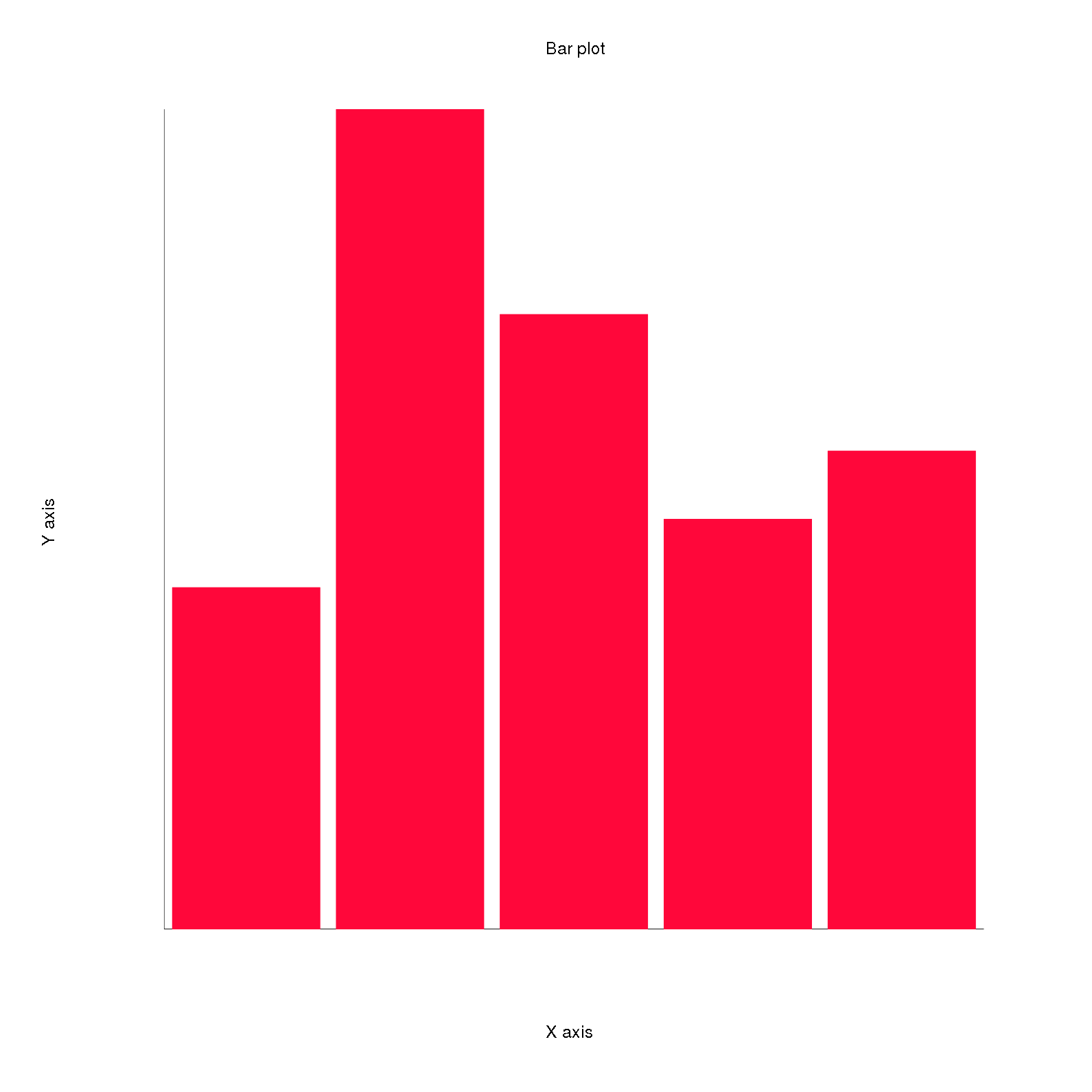
The bar plot draws bars which are rectangles with heights as the data given as the input.
Th inputs taken are the color of the bars(color), the label of the plot(label), the data which is a single array for the sizes of the bars representing the Y values of the bars(data) and the space between the bars as a ratio(spacing_ratio) i.e. the range is [0,1] where 0 represents no space between the bars and 1 represents maximum space between the bars which is equivalent to the maximum space alloted to a bar i.e. (total X range / number of bars).
The X values for the coordinates are set as 0,1,…number of Y values i.e. in this example when the data is given as [5,12,9,6,7], the coordinates for the bars are (0,5), (1,12), (2,9), (3,6) and (4,7) respectively.

Now, the bars are rectangles which are stored in the rectangles array, the X and Y coordinates of lower left corner of these rectangles are stored in abs_x_left and abs_y_left respectively. The upper right corner coordinates are calculated by adding the width of the bar to the X coordinate of the lower left corner and seeting the Y coordinate to the height of the bar as set in the data by the user.
This is done when draw is called which calls the setup_bar_rectangles function:

def draw
  setup_bar_rectangles
  @rectangles.each(&:draw)
end

def setup_bar_rectangles
@data[:y_values].each_with_index do |iy, i|
  @rectangles << Rubyplot::Artist::Rectangle.new(
    self,
    x1: @abs_x_left[i],
    y1: @abs_y_left[i],
    x2: @abs_x_left[i] + @bar_width,
    y2: iy,
    border_color: @data[:color],
    fill_color: @data[:color]
  )
end

This calculation of abs_x_left and abs_y_left is done by the multibars code which will be explained in the next blog.

The draw function of the Ractangle object is:

def draw
  Rubyplot.backend.draw_rectangle(
    x1: @x1,
    y1: @y1,
    x2: @x2,
    y2: @y2,
    border_color: @border_color,
    fill_color: @fill_color,
    abs: @abs
  )
end

It calls the draw_rectangle backend function and passes the information about the rectangle:

def draw_rectangle(x1:,y1:,x2:,y2:, border_color: :default,
  fill_color: nil, border_width: 1, border_type: nil, abs: false)
  within_window(abs) do
    x1 = transform_x(x: x1, abs: abs)
    x2 = transform_x(x: x2, abs: abs)
    y1 = transform_y(y: y1, abs: abs)
    y2 = transform_y(y: y2, abs: abs)

    @draw.stroke Rubyplot::Color::COLOR_INDEX[border_color]
    @draw.fill Rubyplot::Color::COLOR_INDEX[fill_color] if fill_color
    @draw.stroke_width border_width.to_f
    # if fill_color is not given, the rectangle fill colour is transparent
    # i.e. only edges are visible
    @draw.fill_opacity 0 unless fill_color
    @draw.rectangle x1, y1, x2, y2
    @draw.fill_opacity 1 unless fill_color
  end
end

Here, first the coordinates are transformed and then the properties of the rectangle are set and if fill_color is not given then a hollow rectangle is drawn by setting the fill_opacity to 0. Finally, Magick::Draw’s rectangle function is used to draw the rectangle. If the fill_color is not given then the fill_opacity is reset to 1.

Bubble plot

An example of Bubble plot with code is:

@figure = Rubyplot::Figure.new
axes = @figure.add_subplot! 0,0
axes.bubble! do |p|
  p.data [-1, 19, -4, -23], [-35, 21, 23, -4], [4.5, 1.0, 2.1, 0.9]
  p.label = "apples"
  p.color = :blue
end
axes.x_range = [-40, 30]
axes.y_range = [-40, 25]
axes.title = "simple bubble plot."
@figure.write('bubbleplot.png')

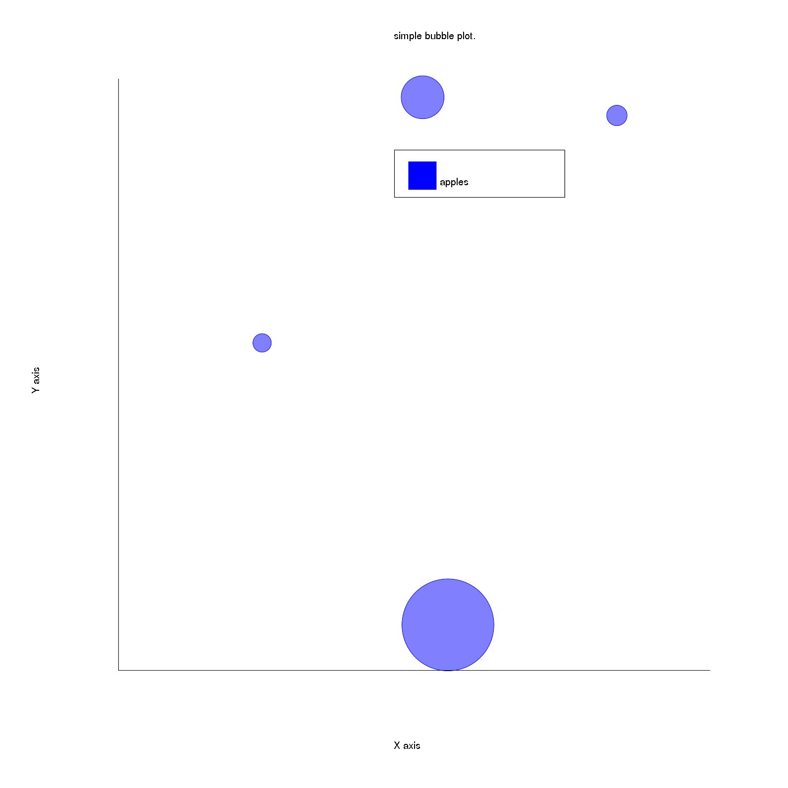
The bubble plot draws circles with the size and the coordinates as specified by the user.
The inputs taken are the data which consists of three arrays for X coordinates, Y coordinates and the sizes of the bubbles respectively(data), the label of the plot(label) and the color of the bubbles(color).

In this example the X,Y coordinates and sizes for the bubbles respectively are (-1, -35), size = 4.5; (19 21), size = 1.0; (-4, 23), size = 2.1; (-23, -4), size = 0.9. The draw function creates and draws the Circle objects for the bubbles:

def draw
  @data[:x_values].each_with_index do |_, idx|
    Rubyplot::Artist::Circle.new(
      self,
      x: @data[:x_values][idx],
      y: @data[:y_values][idx],
      radius: @data[:z_values][idx],
      fill_opacity: 0.5,
      color: @data[:color],
      border_width: 1,
      abs: false
    ).draw
  end
end

Here, for bubble plot, the border width of the circles is set to 1 pixel. The opacity of the circles is hardcoded to 0.5 for visibility of overlapping bubbles.
P.S. - Later, the opacity of the bubble will be taken as an optional input(fill_opacity) with the default value set to 0.5.

The draw function for the Circle object is:

def draw
  Rubyplot.backend.draw_circle(
    x: @x,
    y: @y,
    radius: @radius,
    border_type: :solid,
    border_width: @border_width,
    fill_color: @color,
    border_color: @color,
    fill_opacity: @fill_opacity
  )
end

It calls the backend function draw_circle and passes the information about the circle:

def draw_circle(x:, y:, radius:, border_type: nil, border_width: 1.0, fill_color: nil,
  border_color: :default, fill_opacity: 0.0)
  within_window do
    x = transform_x x: x
    y = transform_y y: y

    @draw.stroke_width border_width
    @draw.stroke Rubyplot::Color::COLOR_INDEX[border_color]
    @draw.fill Rubyplot::Color::COLOR_INDEX[fill_color] if fill_color
    @draw.fill_opacity fill_opacity
    @draw.circle(x,y,x - (radius * NOMINAL_FACTOR_CIRCLE),y)
  end
end

First the coordinates are transformed, then the properties of the circle are set and finally the Magick::Draw’s circle function is called to draw the circle.
Here the radius of the circle is multiplied by a nominal factor in order to match the Magick backend and GR backend sizes. The nominal factor NOMINAL_FACTOR_CIRCLE is hardcoded to 27.5.

Candle-stick plot

An example of Candle-stick plot with code is:

@figure = Rubyplot::Figure.new
axes = @figure.add_subplot! 0,0
axes.candle_stick! do |p|
  p.lows = [100, 110, 120, 130, 120, 110]
  p.highs = [140, 150, 160, 170, 160, 150]
  p.opens = [110, 120, 130, 140, 130, 120]
  p.closes = [130, 140, 150, 160, 150, 140]
end
axes.title = "Simple candle stick plot."
@figure.write('candlestickplot.png')

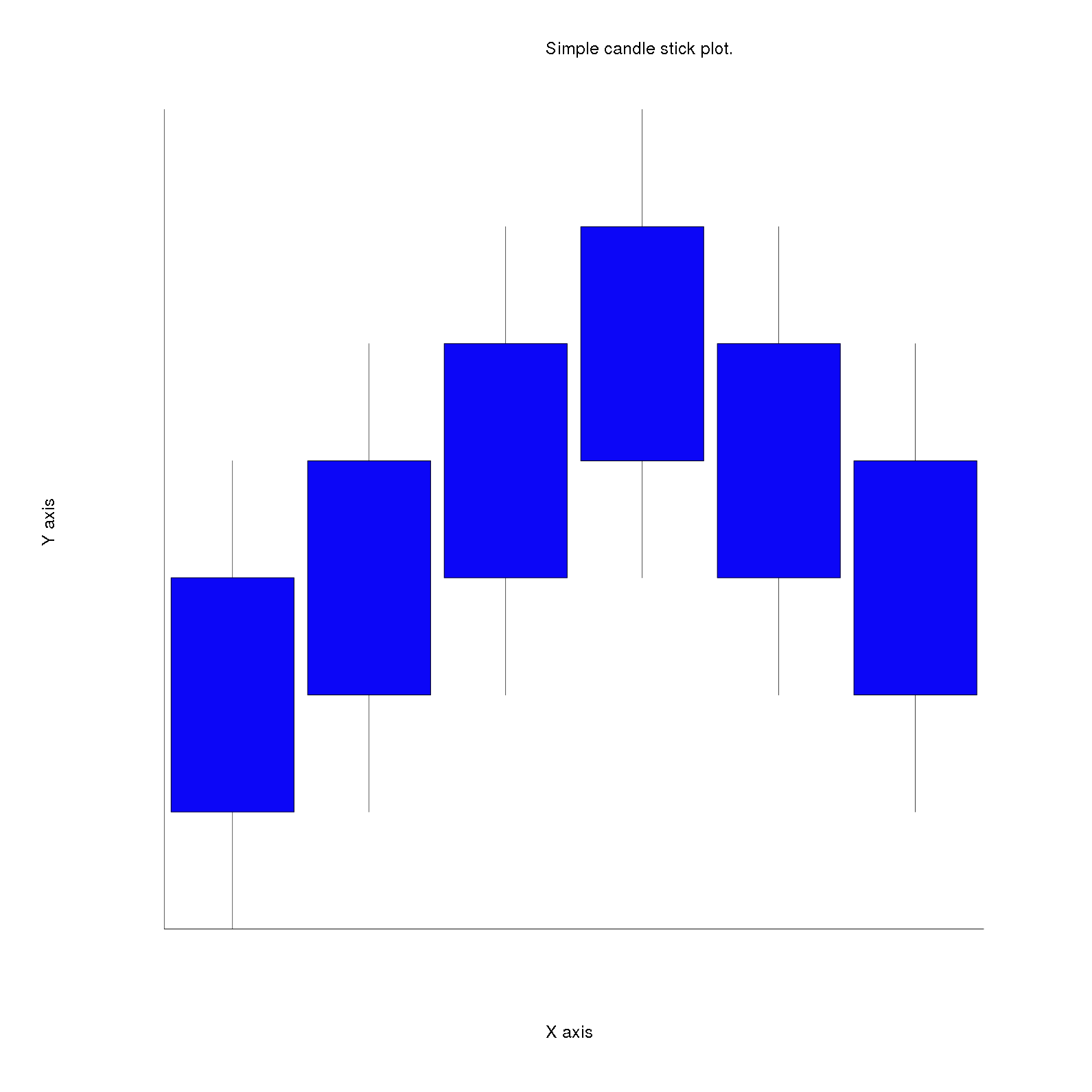
The candle-stick plot draws rectangles i.e. bars (candle) with a line (stick) passing through the center of the rectangles parallel to the Y axis.
The inputs taken are arrays for lower Y coordinate of the rectangles(opens) and upper Y coordinate of the rectangles(closes), arrays for lower Y coordinate of the lines(lows) and the upper Y coordinate of the lines(highs), the colour of the rectangles(color), width of the rectangles(bar_width), the label of the plot(label) and the color of the border of the bars(border_color).

The X coordinates of the lower left corner of the bar and the line are stored in x_left_candle and x_low_stick respectively. The draw function calculates the remaining dimensions (similar to the Bar plot) of the lines and rectangles and creates and draws the Line2D and Rectangle objects for lines and rectangles respectively:

def draw
 @x_low_stick.each_with_index do |ix_stick, i|
   Rubyplot::Artist::Line2D.new(
     self,
     x: [ix_stick, ix_stick],
     y: [@lows[i], @highs[i]]
   ).draw
 end
 
 @x_left_candle.each_with_index do |ix_candle, i|
   Rubyplot::Artist::Rectangle.new(
     self,
     x1: ix_candle,
     y1: @opens[i],
     x2: ix_candle + @bar_width,
     y2: @closes[i],
     border_color: @border_color,
     fill_color: @data[:color]
   ).draw
 end
end

The x_left_candle and x_low_stick are calculated using the multi_candle_stick code which will be explained in the next blog.

The Rectangle object is explained previously. For, the line(stick), a Line2D object is created and drawn with default colour which is black. The Line2D object is a straight line between two points. The draw function for Line2D is:

def draw
  Rubyplot.backend.draw_lines(x: @x, y: @y,
    width: @width, color: @color, opacity: @opacity, type: @type)
end

This passes the properties of the line to the backend function draw_lines, which is:

def draw_lines(x:, y:, width: 2.0, type: :default, color: :default, opacity: 1.0)
  within_window do
    y.each_with_index do |_, idx_y|
      if idx_y < (y.length - 1)
        x1 = transform_x(x: x[idx_y], abs: false)
        y1 = transform_y(y: y[idx_y], abs: false)
        x2 = transform_x(x: x[idx_y + 1], abs: false)
        y2 = transform_y(y: y[idx_y + 1], abs: false)
        LINE_TYPES[type].call(@draw, x1, y1, x2, y2, width, color, opacity)
      end
    end
  end
end

It iterates over the array of X values and Y values and draws straight lines between the consecutive points i.e. the current point and the point stored in the next index of the arrays. After transforming the points, based on the line type, the values are passed to a hash of lambdas(just like scatter plot markers) for drawinf the line. The hash is:

LINE_TYPES = {
  # Default type is solid
  default: ->(draw, x1, y1, x2, y2, width, color, opacity) {
    draw.fill_opacity opacity
    draw.stroke_width width
    draw.fill Rubyplot::Color::COLOR_INDEX[color]
    draw.line x1, y1, x2, y2
  },
  solid: ->(draw, x1, y1, x2, y2, width, color, opacity) {
    draw.fill_opacity opacity
    draw.stroke_width width
    draw.fill Rubyplot::Color::COLOR_INDEX[color]
    draw.line x1, y1, x2, y2
  },
  dashed: ->(draw, x1, y1, x2, y2, width, color, opacity) {
    raise NotImplementedError, 'This line has not yet been implemented'
  }
  # Rest of the code omitted due to space constraint
}

Each of these lambdas take the properties of the lines and draw it.

The line types available are solid, dashed, dotted, dashed_dotted, dash_2_dot, dash_3_dot, long_dash, long_short_dash, spaced_dash, spaced_dot, double_dot and triple dot. The default type of line is solid.
Till now, only solid line type is implemented for Magick backend, rest all will be implemented soon.

Hence, the Rectangle and Line2D objects are drawn which are the candle and the stick respectively.

Histogram

An example of Histogram with code is:

@figure = Rubyplot::Figure.new
axes = @figure.add_subplot! 0,0
axes.histogram! do |p|
  p.x = 100.times.map{ rand(10) }
end
@figure.write('histogram.png')

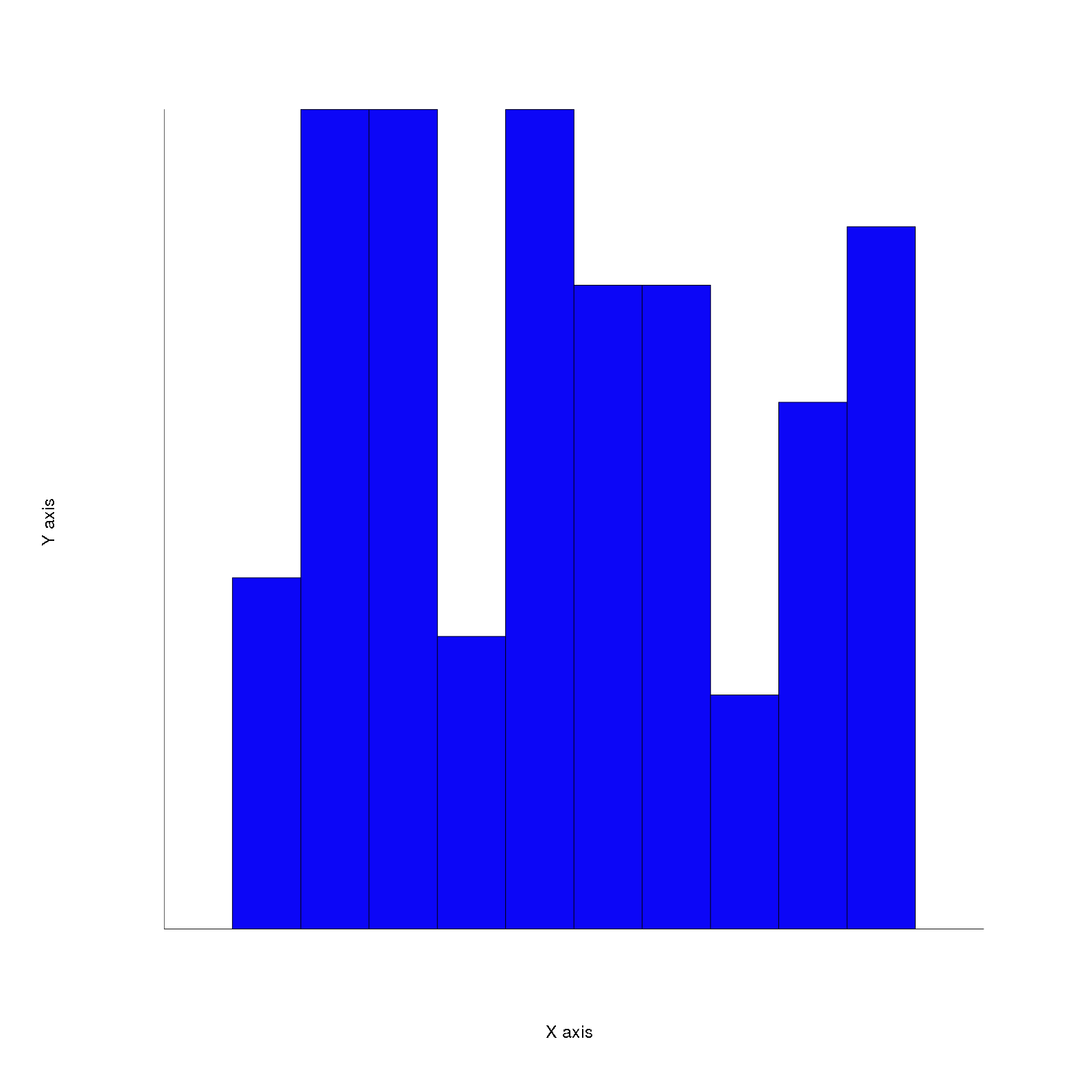
Histogram draws rectangles(bars) which represent the frequency of a label(i.e. an object, a range of numbers, etc.)
The inputs taken are the color of the bars(color), the label of the plot(label), width of the bars(bar_width), an array of numbers as the data(x), an optional number representing number of bins or an array of increasing numbers representing bins over which the frequency will be calculated(bins).

So, bins can be set in three ways:

1. If bins are not specified i.e. not given as an input then number of bins are set as number of unique numbers in the data, here in the example(assuming each number from 0 to 9 is present) the number of bins will be 10. The subdivisions(Integer) is calculated which is the difference maximum value and minimum value in data divided by the number of bins. So, here in the example subdivisions = (9-0)/10 = 0.9 = 0 (as subdivisions is an Integer).
   Then the bins array is set as an array having numbers starting from the minimum value in the data added with subdivisions over and over again until the maximum value in the data and finally the largest unique number added with ubdivisions is appended to the bins array. So, the bins array is [0, 1, 2, 3, 4, 5, 6, 7, 8, 9, 10] and hence the bins are 0-1, 1-2, 2-3, 3-4, 4-5, 5-6, 6-7, 7-8, 8-9 and 9-10. The bins are inclusive of the starting number.
2. If bins are given as the number of bins i.e. an Integer representing the number of bins then similarly to case 1, the bins are calculated.
3. If bins are given directly i.e. an array is given.
   Example - [1,4,7,10] then the bins will be [1,4), [4,7), [7,10] i.e. the startig value is included and the ending value is excluded unless it’s the end of values i.e. bins array.

After calculating the bins, the combined frequencies of the bins are calculated which are the heights of the bars for each bin. Hence, the Rectangle objects are drawn(as explained previously) with each bar representing a bin and the height representing the frequency of the bin.

Line plot

An example of Line plot with code is:

@figure = Rubyplot::Figure.new
axes = @figure.add_subplot! 0,0
axes.line! do |p|
  p.data [2, 4, 7, 9], [1,2,3,4]
  p.label = "Marco"
  p.color = :blue
end
axes.title = "A line graph."
@figure.write('lineplot.png')

The Line plot draws a line between consecutive points specified by the user and thus draws a line passing through the points taken as input.
The input taken by the Line plot are type of the line(line_type), width of the line(line_width), the color of the line(line_color) and the data having a compulsory array having Y coordinate values for the points and an optional array having X coordinate values(data) and the label of the plot(label).

If only one array is given to the line plot as the data then the X coordinate values are calculated as 0,1,2…(number of Y - 1) values. This is similar to the Area plot.

The draw function calls the draw_lines backend function to create the lines, which is as explained before and hence the Line plot is drawn.

Error-bar plot

An example of Error-bar plot with code is:

@figure = Rubyplot::Figure.new
axes = @figure.add_subplot! 0,0
axes.title = "Simple error bar plot with collection xerr and yerr."
axes.error_bar! do |p|
  p.data [1,2,3,4], [1,4,9,16]
  p.xerr = [0.5,1.0,1.5,0.3]
  p.yerr = [0.6,0.2,0.8,0.1]
end
@figure.write('errorbarplot.png')

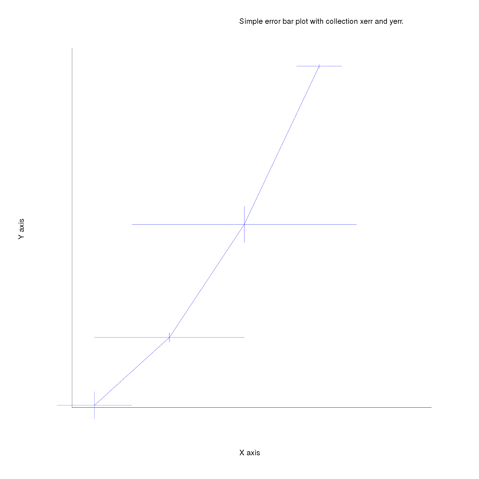
Error-bar plot draws a line plot for the data taken and draws lines for errors at the given points.
The inputs taken are two arrays for X coordinate values and Y coordinate values respectively(data), label of the plot(label), colour of the line and the error lines(color), an array for X error values(xerr) and an array for Y error values(yerr).

The line and the errors are all Line2D objects which are explained previously. The coordinates for the error lines are calculated by adding and subtraicting the error to the coordinates i.e. suppose at the first point (1,1) the X error is 0.5 then the X error line will be between the points (0.5,1) and (0.5,1) and similarly the Y error is 0.6 then the Y error line is between the points (1,0.4) and (1,1.6).

Box plot

An example of Box plot with code is:

figure = Rubyplot::Figure.new
axes = @figure.add_subplot! 0,0
axes.title = "A simple box plot."
axes.box_plot! do |p|
  p.data [
    [60,70,80,70,50],
    [100,40,20,80,70],
    [30, 10]
  ]
end
axes.x_title = "foo"
axes.y_title = "bar"
@figure.write('boxplot.png')

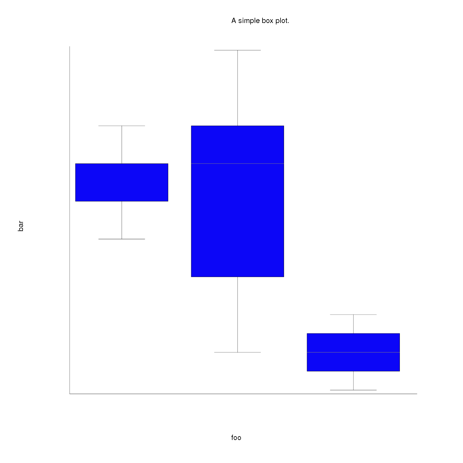
The box plot will be explained in the next blog in the multi box plot section.